10. Backpropagation- Example (part b)
Backpropagation- Example (part b)
Now that we understand the chain rule, we can continue with our backpropagation example, where we will calculate the gradient
12 Backpropagation Example B V6 Final
In our example we only have one hidden layer, so our backpropagation process will consist of two steps:
Step 1: Calculating the gradient with respect to the weight vector W^2 (from the output to the hidden layer).
Step 2: Calculating the gradient with respect to the weight matrix W^1 (from the hidden layer to the input).
Step 1
(Note that the weight vector referenced here will be W^2. All indices referring to W^2 have been omitted from the calculations to keep the notation simple).
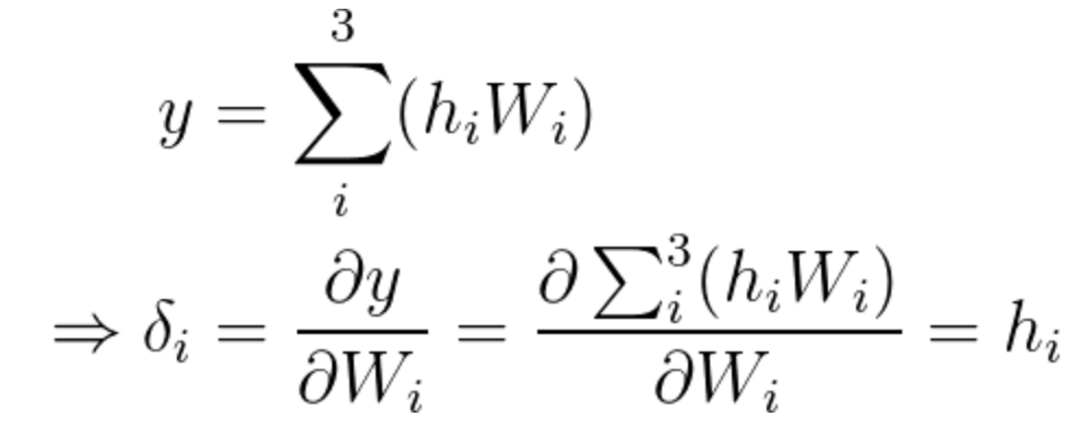
Equation 13
As you may recall:
\large\Delta W_{ij}=\alpha(d-y) \frac{\partial y}{\partial W_{ij}}
In this specific step, since the output is of only a single value, we can rewrite the equation the following way (in which we have a weights vector):
\large\Delta W_i=\alpha(d-y) \frac{\partial y}{\partial W_i}
Since we already calculated the gradient, we now know that the incremental value we need for step one is:
\Delta W_i=\alpha(d-y) h_i
Equation 14
Having calculated the incremental value, we can update vector W^2 the following way:
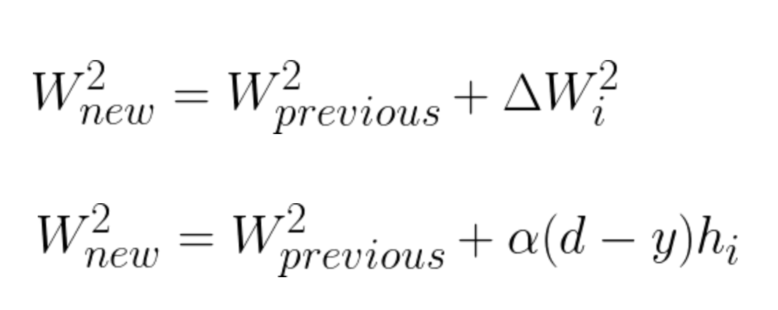
Equation 15
Step 2
(In this step, we will need to use both weight matrices. Therefore we will not be omitting the weight indices.)
In our second step we will update the weights of matrix W^1 by calculating the partial derivative of y with respect to the weight matrix W^1.
The chain rule will be used the following way:
obtain the partial derivative of y with respect to \bar{h}, and multiply it by the partial derivative of \bar{h} with respect to the corresponding elements in W^1. Instead of referring to vector \bar{h}, we can observe each element and present the equation the following way:
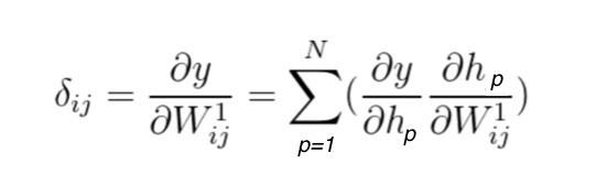
Equation 16
In this example we have only 3 neurons the the single hidden layer, therefore this will be a linear combination of three elements:
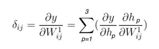
Equation 17
We will calculate each derivative separately. \frac{\partial y}{\partial h_j} will be calculated first, followed by \frac{\partial h_j}{\partial W^1_{ij}}.
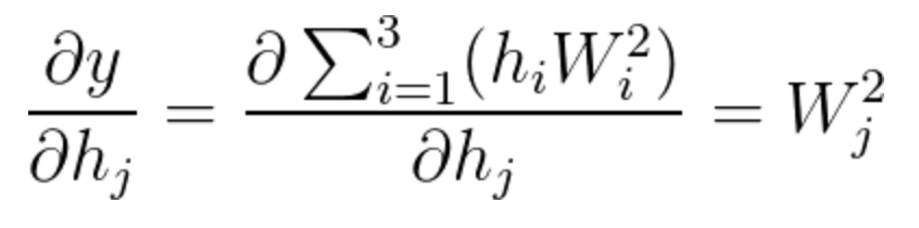
Equation 18
Notice that most of the derivatives were zero, leaving us with the simple solution of \frac{\partial y}{\partial h_{j}}=W^2_j
To calculate \frac{\partial h_j}{\partial W^1_{{ij}}} we need to remember first that
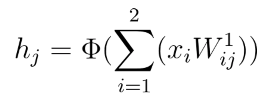
Equation 19
Therefore:
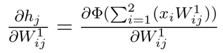
Equation 20
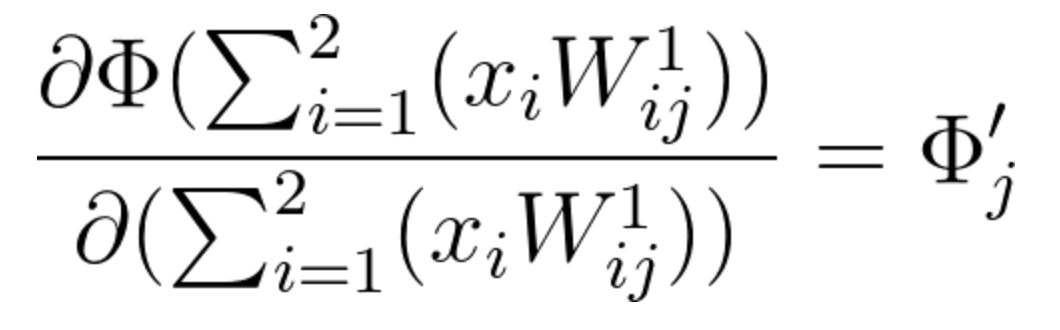
Since the function \ h_j is an activation function (\Phi) of a linear combination, its partial derivative will be calculated the following way:
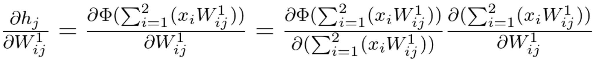
Equation 21
Given that there are various activation functions, we will leave the partial derivative of \Phi using a general notation. Each neuron j will have its own value for \Phi and \Phi', according to the activation function we choose to use.
Equation 22
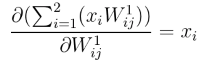
The second calculation of equation 21 can be calculated the following way:
(Notice how simple the result is, as most of the components of this partial derivative are zero).
Equation 23
After understanding how to treat each multiplication of equation 21 separately, we can now summarize it the following way:
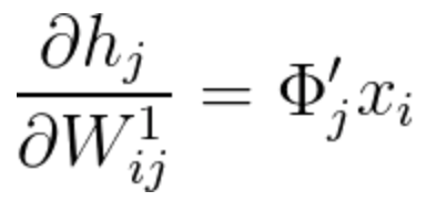
Equation 24
We are ready to finalize step 2, in which we update the weights of matrix W^1 by calculating the gradient shown in equation 17. From the above calculations, we can conclude that:
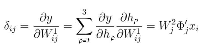
Equation 25
Since \Delta W^1_{ij}=\alpha(d-y) \large\frac{\partial y}{\partial W^1_{ij}} , when finalizing step 2, we have:
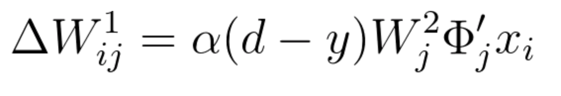
Equation 26
Having calculated the incremental value, we can update vector W^1 the following way:
W^1_{new}=W^1_{previous}+\Delta W^1_{ij}
W^1_{new}=W^1_{previous}+\alpha(d-y)W^2_j\Phi'_jx_i
Equation 27
After updating the weight matrices we begin once again with the Feedforward pass, starting the process of updating the weights all over again.
This video touches on the subject of Mini Batch Training. We will further explain things in our Hyperparameters lesson coming up.